
This step by step guide show you how to perform a regression analysis in Excel and how to interpret the Summary Output.
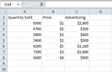
Below you can find our data. The big question is: is there a relation between Quantity Sold (Output) and Price and Advertising (Input). In other words: can we predict Quantity Sold if we know Price and Advertising?
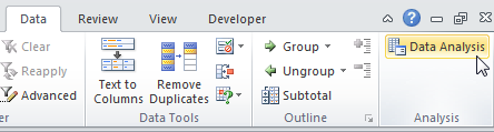
1. On the Data tab, click Data Analysis.

Note: If you can't find the Data Analysis button? Follow "How to Load Analysis ToolPak add-in"
steps mentioned in the end of this post to load it.
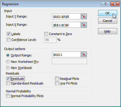
2. Select Regression and click OK.

3. Select the Y Range (A1:A8). This is the predictor variable (also called dependent variable).
4. Select the X Range(B1:C8). These are the explanatory variables (also called independent variables).
These columns must be adjacent to each other.
5. Check Labels.
6. Select an Output Range.
7. Check Residuals.
8. Click OK.
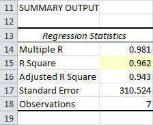
Excel produces the following Summary Output (rounded to 3 decimal places).
R Square
R Square equals 0.962, which is a very good fit. 96% of the variation in Quantity Sold is explained by the independent variables Price and Advertising. The closer to 1, the better the regression line (read on) fits the data.
Significance F and P-values
To check if your results are reliable (statistically significant), look at Significance F (0.001). If this value is less than 0.05, you're OK. If Significance F is greater than 0.05, it's probably better to stop using this set of independent variables. Delete a variable with a high P-value (greater than 0.05) and rerun the regression until Significance F drops below 0.05.
Most or all P-values should be below below 0.05. In our example this is the case. (0.000, 0.001 and 0.005).
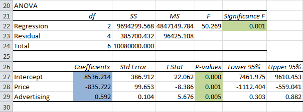
Coefficients
The regression line is: y = Quantity Sold = 8536.214-835.722 * Price + 0.592 * Advertising. In other words, for each unit increase in price, Quantity Sold decreases with 835.722 units. For each unit increase in Advertising, Quantity Sold increases with 0.592 units. This is valuable information.
You can also use these coefficients to do a forecast. For example, if price equals $4 and Advertising equals $3000, you might be able to achieve a Quantity Sold of 8536.214 -835.722 * 4 + 0.592 * 3000 = 6970.
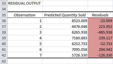
Residuals
The residuals show you how far away the actual data points are fom the predicted data points (using the equation). For example, the first data point equals 8500. Using the equation, the predicted data point equals 8536.214 -835.722 * 2 + 0.592 * 2800 = 8523.009, giving a residual of 8500 - 8523.009 = -23.009.
You can also create a scatter plot of these residuals.

How to Load Analysis ToolPak add-in
The Analysis ToolPak is an Excel add-in program that provides data analysis tools for financial, statistical and engineering data analysis.To load the Analysis ToolPak add-in, execute the following steps.
1. Click on the green File tab. The File tab in Excel 2010 or later replaces the Office Button (or File Menu) in previous versions of Excel.
2. Click on Options.

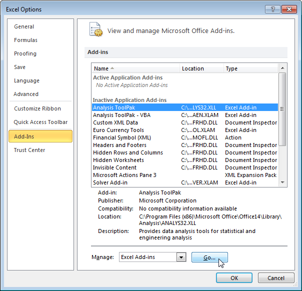
3. Under Add-ins, select Analysis ToolPak and click on the Go button.
4. Check Analysis ToolPak and click on OK.

5. On the Data tab, you can now click on Data Analysis.
The following dialog box below appears.
6. For example, select Histogram and click OK to create a Histogram in Excel.
